Learning

• Basic concepts
• Learning a decision tree (Quinlan's method
• Rough sets
• General concepts
• Potential applications
• Another look at neural networks based on these concepts
• Components of a learning agent (reading, chapter 18 upto page 531)
  • supervised learning
    • you (supervisor) know the correct answer
    • the agent tries to adjust its prediction method based on the feedback
  • reinforcement
    • evaluation of action
    • there may not be a right answer but a cost associated with the chose action
  • unsupervised learning
    • figure out patterns on your own and use the paterns in some meaningful way
• Decision trees
  • Decision tree given in Fig. 18.4 describes the decisions that will be made by a person regarding waiting for a seat in the restaurant
  • You can follow any path and construct a logical sentence that will determine whether or not the person will wait.
  • What type of logic is expressible by the decision tree?
  • You cannot have real relations in a decision tree, so it is essentially propositional logic.
• Page 534: shows a table of examples that is created from the decision tree.
• Generally, we start with the examples and then build the decision tree.
• Data mining is becoming a very popular area of application for learning
• Most of the major stores give you incentives to use their card such and A&P
• This data can be processed with the faster computers
• There is no evidence that they are actually doing anything significant with the data.
• Given a table find a decision tree: preferably simplest
• Algorithm (page 535):
  • choose an attribute that will provide the best classification of the objects in the table
  • The ultimate classification will be the one that correponds to minimum entropy. That is based on the value of attribute we can make decision about the classification
  • Generally perfect classification using a single attribute is not possible
  • Fig. 18.6 a versus b, patrons clearly seems like the best of the two.
  • So we start the decision tree with patrons. If the value for patron is full, we cannot conclude anything.
  • So we move on and select next attribute (hungry?)
  • The process continues, results are shown in Fig 18.8
  • The tree that was learned was better than original tree
• Generally, databases are too big for a human to identify the patterns. Computers as naive as they are can go through all the patterns systematically.
• Examples of real life applications on page 539-540.
• How do we decide which one is the best attribute?
• Information theory:

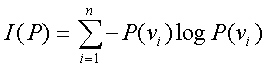
• This is also known as entropy.
• Let us calculate gain(patron)
  • P(none)=2/12,I(none)=0
  • P(some)=4/12,I(some)=0
  • P(full)=6/12
    • we have 6 examples 2 positive and 4 negative
    • 2/6=1/3,4/6=2/3
    • I(full)=0.918
  • expected information called remainder(patron)
  • p(none)*i(none)+p(some)*i(some)+p(full)*i(full)
  • 0+0+0.5*0.918
  • 0.459
  • gain(patron)=original-remainder(patron)
  • 0.541
  • Similarly, you can calculate gain(type) on page 541 is show to be equal to 0
  • Choose the attribute with highest gain
• We can use other statistical measures to identify irrelevant attributes. Read pages 542-543.
• Decision trees can be exponential. May not always be the best knowledge representations
• Rough Sets, Pawlak (1984)

Id	Headache	Mucsle-pain	Temp.	Flu
p1	no	yes	high	yes
p2	yes	no	high	yes
p3	yes	yes	veryhigh	yes
p4	no	yes	normal	no
p5	yes	no	high	no
p6	no	yes	veryhigh	yes

• We want to determine rules that will tell us whether the patient has flue depending on the attributes headache, muscle-pain, fever
• You can construct an equivalence relation using the evidence attributes. If two objects have excatly the same values for all the attributes then they are in the same equivalence class.
• set for flue = {p1,p2,p3,p6}
• notflue={p4,p5}
• lower(flue)={p1,p3,p6}
• upper(flue)={p1,p2,p3,p5,p6}
• lower(notflue)={p4}
• upper(notflue)={p2,p4,p5}
• These upper and lower bounds can be used to determine IF...THEN type of rules
• We can also use different probability cut-offs to eliminate odd noise in the data
• Reduct allows you to choose only the relevant attribute
  • verify that using only headache and temp may be sufficient to get the same results
  • similarly, using only muscle-pain and temp may be sufficient to get the same results
• Assessing the performance of the learning algorithm
• Divide your set of examples into training and test set.
• Develop the strategy using training set and then apply it to test set
• Many times during debugging the program is fixed based on how it performed for the test set. The test set gets tainted because it is used in developing the strategy.
• Figure 18.9 shows how the performance changes with the size of the train and test set.
• Generally, we will go with the knee-of-curve approach
• In the figure 20 may be a good size for the training set.
• Pages 546-550: Definition of
  • current-best-hypothesis search
  • Find a single hypothesis which explains all the positive examples
    • incremental learning with new examples
    • false positive: algo says positive but in reality it is negative
    • Specialize
    • Figure 18.10(d&e)
    • false negative: algo says negative but in reality it is positive
    • generalize
    • Figure18.10(b&c)
  • Least commitment search
  • Start with a huge hypothesis space and eliminate individual hypothesis as we see false positive or negative examples
  • Exponential
• Neural networks
  • Supervised learning
  • We know the answer. We try to find a function that will predict the answer by adjusting the weights
  • Unsupervised learning
  • Kohonen rule
  • Given a set of patterns, separate them into different classes. The values of classes are not known. Kohonen network will classify on its own